How to change partition column in dbt incrementally without losing any data in BigQuery

When working with dbt, sometimes you deal with data partitioned by a non-relevant column, such as the ingestion time. In order to make queries faster and cheaper, you need to partition the table by the field by which you want to filter your queries.

In this article, I will explain how changing the partition column may cost you losing data, why dbt incremental produces this outcome, and how to avoid this loss completely. We will use Google Cloud’s billing data to exemplify this problem.

Dataset analysis

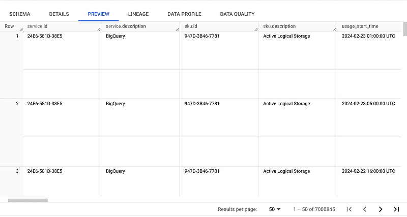
GCP’s billing export is composed of three tables: the pricing table, the standard report table, and the detailed report table. When you define where you want these data to be exported, these tables will be created and Google will start ingesting billing data regularly. In the image below you can see a small portion of the available columns on the detailed report table.

This table is partitioned by the special column called _PARTITIONTIME. This column is only created when you specify that you want your data to be partitioned by the time it was ingested. It is worth mentioning that this column does not appear in the schema but you can query it.

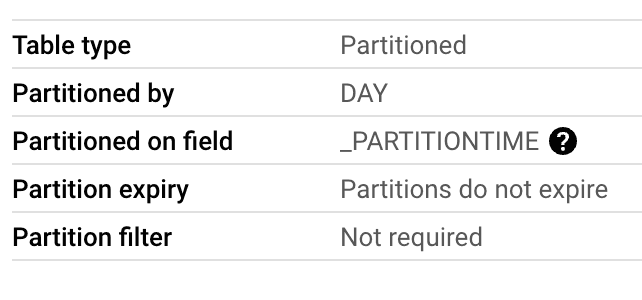
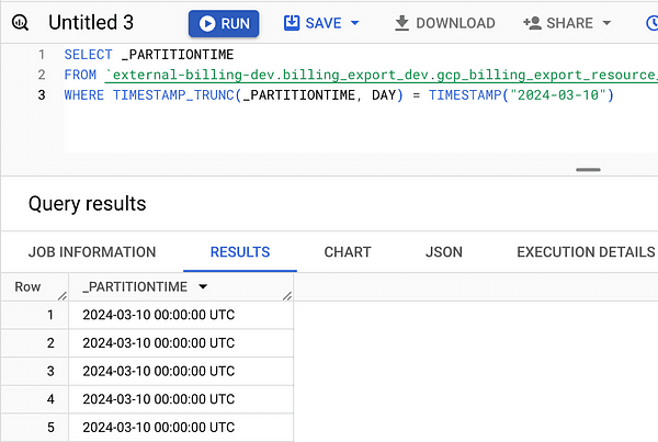
Detailed pricing table and its partition _PARTITIONTIME

Each row represents a cost produced in Google Cloud, which has a starting time of usage and an ending time. This may not seem like an issue at first, but the ingested time is not always the equivalent of the time when the cost was produced.

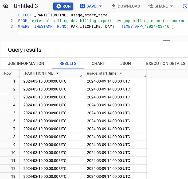
Difference between _PARTITIONTIME and usage_start_time

You may be wondering what is the issue about having a different partition date than the date when the charge was incurred. Let’s compare the cost of a query on the ingested time and the time when the usage was consumed.

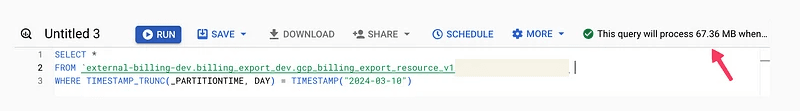
Cost when filtering by ingested time (67.36 MB)

Cost when filtering by the date where the cost was produced (6.35 GB)

We can see in the two examples that querying the actual consumed date is 100 times as much processing as simply querying by the ingested time (which also means 100 times more expensive). This is an issue because we want to know the costs on a given day, not the cost of the ingested data on a given day.

For this reason, we want to change the partition of the table from _PARTITIONTIME to usage_start_time. And this is where the real problem begins.

Losing data because of partition column change

Straightforward approach

The first approach we will follow is having a simple query that just gets all the data from the source table to the destination table changing the partition to usage_start_time.

{{
    config(
        materialized = 'incremental',
        incremental_strategy='insert_overwrite',
        partition_by = {
            "field": "usage_start_time",
            "data_type": "timestamp",
            "granularity": "day"
        },
        on_schema_change='fail'
    )
}}

select * from {{ source('billing_export', 'gcp_billing_export_resource') }}
  {% if is_incremental() %}
    WHERE TIMESTAMP_TRUNC(_PARTITIONTIME, DAY) = TIMESTAMP('2024-01-05') 
  {% endif

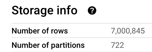
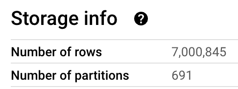
We first run the model to get the table partitioned by our new field. No problem so far. Before running this query, we have a total number of rows of 7.000.845. Let’s see what happens after we run the given query (with today’s date).

After running our incremental query on this date (05–01–2004), we get the following:

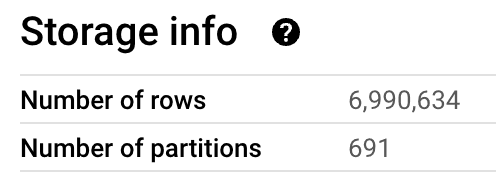
Wait, what? How come we have lost rows by running the model incrementally? To answer that question we need to dive into how dbt incremental insert_overwrite strategy works.

This strategy runs two queries, the first one creates a temporary table with the data from our query, you can see the query below.

create or replace table `external-billing-dev`.`test`.`usage_partition__dbt_tmp`
      
    partition by timestamp_trunc(usage_start_time, day)

    OPTIONS(
      description="""""",
    
      expiration_timestamp=TIMESTAMP_ADD(CURRENT_TIMESTAMP(), INTERVAL 12 hour)
    )
    as (

select * from `external-billing-dev`.`billing_export_dev`.`gcp_billing_export_resource_v1_...`
  
    WHERE TIMESTAMP_TRUNC(_PARTITIONTIME, DAY) = TIMESTAMP('2024-01-05') 
  
    )

Until this point, everything looks normal. The query ran with the where statement so there were barely any costs out of this query (Bytes processed = 3.35 MB). Let’s see the second query done by dbt.

-- generated script to merge partitions into `external-billing-dev`.`test`.`usage_partition`
declare dbt_partitions_for_replacement array<timestamp>;

    
    
-- 1. temp table already exists, we used it to check for schema changes
-- 2. define partitions to update
set (dbt_partitions_for_replacement) = (
    select as struct
        -- IGNORE NULLS: this needs to be aligned to _dbt_max_partition, which ignores null
        array_agg(distinct timestamp_trunc(usage_start_time, day) IGNORE NULLS)
    from `external-billing-dev`.`test`.`usage_partition__dbt_tmp`
);

-- 3. run the merge statement

merge into `external-billing-dev`.`test`.`usage_partition` as DBT_INTERNAL_DEST
    using (
    select
    * from `external-billing-dev`.`test`.`usage_partition__dbt_tmp`
    ) as DBT_INTERNAL_SOURCE
    on FALSE

when not matched by source
        and timestamp_trunc(DBT_INTERNAL_DEST.usage_start_time, day) in unnest(dbt_partitions_for_replacement) 
    then delete

when not matched then insert
    (`billing_account_id`, `service`, `sku`, `usage_start_time`, `usage_end_time`, `project`, `labels`, `system_labels`, `location`, `resource`, `export_time`, `cost`, `currency`, `currency_conversion_rate`, `usage`, `credits`, `invoice`, `cost_type`, `adjustment_info`, `tags`, `price`, `cost_at_list`, `transaction_type`, `seller_name`, `subscription`)
values
    (`billing_account_id`, `service`, `sku`, `usage_start_time`, `usage_end_time`, `project`, `labels`, `system_labels`, `location`, `resource`, `export_time`, `cost`, `currency`, `currency_conversion_rate`, `usage`, `credits`, `invoice`, `cost_type`, `adjustment_info`, `tags`, `price`, `cost_at_list`, `transaction_type`, `seller_name`, `subscription`)

;

-- 4. clean up the temp table
drop table if exists `external

Let’s check the second statement, where the partitions are selected in this query.

with first_query_table as(
  select * from `external-billing-dev`.`billing_export_dev`.`gcp_billing_export_resource_v1_...`
  WHERE TIMESTAMP_TRUNC(_PARTITIONTIME, DAY) = TIMESTAMP('2024-01-05') 
)
  
select array_agg(distinct timestamp_trunc(usage_start_time, day) )
from

The result is the following

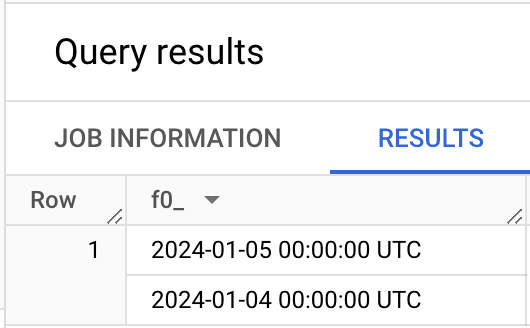
Return from partition query.

So, we ran our model on the 5th of January 2024, but we got that the model was trying to replace the previous day as well. Why is that happening?

Basically, we are telling dbt to get all records of 05–01–2024 on the partition field on the source table. Then, dbt looks for all distinct entries of the partition field on the destination table. Let’s continue looking at the query to understand what happens next.

-- 3. run the merge statement
merge into `external-billing-dev`.`test`.`usage_partition` as DBT_INTERNAL_DEST
    using (
    select
    * from `external-billing-dev`.`test`.`usage_partition__dbt_tmp`
    ) as DBT_INTERNAL_SOURCE
    on FALSE

when not matched by source
        and timestamp_trunc(DBT_INTERNAL_DEST.usage_start_time, day) in unnest(dbt_partitions_for_replacement) 
    then delete

when not matched then insert
    (`billing_account_id`, `service`, `sku`, `usage_start_time`, `usage_end_time`, `project`, `labels`, `system_labels`, `location`, `resource`, `export_time`, `cost`, `currency`, `currency_conversion_rate`, `usage`, `credits`, `invoice`, `cost_type`, `adjustment_info`, `tags`, `price`, `cost_at_list`, `transaction_type`, `seller_name`, `subscription`)
values
    (`billing_account_id`, `service`, `sku`, `usage_start_time`, `usage_end_time`, `project`, `labels`, `system_labels`, `location`, `resource`, `export_time`, `cost`, `currency`, `currency_conversion_rate`, `usage`, `credits`, `invoice`, `cost_type`, `adjustment_info`, `tags`, `price`, `cost_at_list`, `transaction_type`, `seller_name`, `subscription`)
What this merge statement does is the following:

What this merge statement does is the following:

• Create a merge statement to add new rows to `external-billing-dev`.`test`.`usage_partition` from our usage_partition__dbt_tmp table created before.

• On false means that there won’t be any matching entries, which is helpful for the following statements.

• The not matched by source statement will delete any row in the destination table that fulfill the condition, which is: not to be a match (no row is matched because we set it to on false) and that belongs to the partitions that we chose (which we saw in the last code block). Therefore, it deletes ALL rows from days 04–01–24 and 05–01–24.

• The when not matched then insert statement inserts all rows from the source that are not matched with the destination, are inserted in the destination. In practice, this inserts all row from source because we set it the on false condition before.

To summarize, following this approach, dbt looks at all distinct values of the destination table partition column that appear in our query on a given date on the source table partition column. Then, it deletes the whole partitions in the destination table where the values of the destination partition column match. Finally, it inserts the values of the source table into the destination table.

Therefore, the issue is that any row ingested in the source table on any date different than 05–01–2024 which has a usage_start_time on that date, will be removed because we all deleting its entire partition but we are only inserting in the table the data of the 05–01–2024.

The solution

Now that we not the problem, we can find a solution for it. First, let’s define what are our goals.

• We want to ingest all new data from the source table partitioned by ingestion to the table partitioned by usage_start_time.

• We cannot afford losing data on the process. The rows on the source table must be the exactly the same as in the destination table.

To achieve this, we can do the following.

• Check in the source table all distinct usage_start_time dates ingested on a given date. Example: On day 05–01–2024, ingested rows have 2 distinct values of usage_start_time (05–01–2024, 06–01–2024).

• Take all rows in the source table where usage_start_time corresponds to any of those dates.

• Check only recent partitions to avoid scanning the whole table.

With this process, we have the following query:

{{
    config(
        materialized = 'incremental',
        incremental_strategy='insert_overwrite',
        partition_by = {
            "field": "usage_start_time",
            "data_type": "timestamp",
            "granularity": "day"
        },
        on_schema_change='fail'
    )
}}

select * from {{ source('billing_export', 'gcp_billing_export_resource') }}
  {% if is_incremental() %}
    WHERE TIMESTAMP_TRUNC(usage_start_time, DAY) in (
      SELECT distinct TIMESTAMP_TRUNC(usage_start_time, DAY) 
      FROM {{ source('billing_export', 'gcp_billing_export_resource') }}
      WHERE TIMESTAMP_TRUNC(_PARTITIONTIME, DAY) = TIMESTAMP('2024-01-05') 
    )
    AND TIMESTAMP_TRUNC(_PARTITIONTIME, DAY) <= TIMESTAMP(DATE_ADD('2024-01-05', INTERVAL 5 DAY))
    AND TIMESTAMP_TRUNC(_PARTITIONTIME, DAY) >= TIMESTAMP(DATE_SUB('2024-01-05', INTERVAL 2 DAY))  
{% endif

On the first part of the incremental statement, we take all distinct values of usage_start_time where the ingested date is 05–01–2024. Then, we filter the result of the query to only take data from the resulting dates.

WHERE TIMESTAMP_TRUNC(usage_start_time, DAY) in (
      SELECT distinct TIMESTAMP_TRUNC(usage_start_time, DAY) 
      FROM {{ source('billing_export', 'gcp_billing_export_resource') }}
      WHERE TIMESTAMP_TRUNC(_PARTITIONTIME, DAY) = TIMESTAMP('2024-01-05') 
    )

Then, we take a margin of 2 days on the past and 5 days on the future. This statement doesn’t change the result, but it does change the cost of the query. If we don't set it, we will scan the whole table for those rows that fulfill the previous condition. With this new conditions, we only check 8 partitions, which is way faster and cheaper.

AND TIMESTAMP_TRUNC(_PARTITIONTIME, DAY) <= TIMESTAMP(DATE_ADD('2024-01-05', INTERVAL 5 DAY))
AND TIMESTAMP_TRUNC(_PARTITIONTIME, DAY) >= TIMESTAMP(DATE_SUB('2024-01-05', INTERVAL 2 DAY))

You may be wondering: why do you take 5 partitions ahead and 2 back? It depends on the case, but checking the data I saw that sometimes there is old partitions with data of a given day, and also that data is ingested on the coming 5 days. Your case is likely different so make sure to understand when can data from a given day be ingested in your source table. This way you can check the minimum number of partitions to reduce time and cost.

If we execute the query, we get the following result on the destination table.

Conclusion

When I started working with Google Cloud billing data, I went with the first approach explained in the article, which caused a lot of data loss. It was a problem not easy to spot and neither to debug. After some time thinking about a possible solution I ended up with what I showed you as the solution. It allowed me to change the partition of the table incrementally, cheaply and fast.

The worst bugs are those that are silent, which you don’t spot at the moment, which is the case of this one. Luckily I found out and was able to solve it. Imagine running your data pipelines losing data consistently on a daily basis… what a nightmare.

I hope this article showed you how you can deal with this problem and to always be careful when working with dbt incremental. It deletes partitions that it will then insert, unless the data inserted is not the same as the deleted.

Thank you

If you enjoyed reading this article, stay tuned as we regularly publish technical articles on dbt, Google Cloud and how to secure those tools at best. Follow Astrafy on LinkedIn to be notified for the next article ;).

If you are looking for support on Data Stack or Google Cloud solutions, feel free to reach out to us at sales@astrafy.io.